Tuesday Links
- Nick Barnes and colleagues and contributors are off to what looks like a great start with a new open source version of GISTEMP.
- Jeffrey Park from Yale examines the relationship between temperature and CO2 at interannual time scales in Geophysical Research Letters.
Since 1979, at Mauna Loa and other observation sites, interannual coherence exhibits a 90° phase lag that suggests a direct correlation between temperatures and the time-derivative of CO2. The coherence transition can be explained if the response time of CO2 to a global temperature fluctuation has lengthened from 6 months to at least 15 months. A longer response time may reflect saturation of the oceanic carbon sink, but a transient shift in ocean circulation may play a role.
- Naomi Levin and colleagues find a possible source for the high stable isotope values of rainfall in Ethiopia in the Journal of Geophysical Research.
The combination of wind direction data from Ethiopia and
e distribution in Africa indicates that transpired moisture from the Sudd and the Congo Basin is likely responsible for the high isotopic values of rainfall in Ethiopia.
- Andrew Dessler and Sun Wong on ‘Estimates of the Water Vapor Climate Feedback during El Niño–Southern Oscillation‘ in Journal of Climate.
‘Doubt is their product’
An excellent post from Jeff Masters on The Manufactured Doubt Industry.
Happy Thanksgiving, everyone.
On water, climate change, Lomborg, and getting your facts right
Via John Fleck, I found this opinion piece by Bjorn Lomborg on climate change, water, and adaptation in Bangladesh. The main thrust of the article is that if the goal is to reduce the harmful consequences of anthropogenic climate change, resources would be better spent on projects to improve access to the basic necessities of the poor and the developing world in general, rather than on reducing carbon emissions.
Not that it should matter what I think, but in this instance I would agree. I think that improving basic access to clean water, sanitation, health care and nutrition, and infrastructure in the developing world addresses a host of interrelated ethical and moral, social, economic, public health, energy, national security, and environmental issues. I think such resources would be well-spent and substantially enhance the adaptive capacity of countries in the face of future climate change. This is not an either/or proposition, however, — the sense one inevitably gets from Lomborg’s writing and those that subscribe to his particular tactics and approach — increasing adaptive capacity, reducing vulnerability, and reducing emission have to proceed together. There is no one single solution nor policy that addresses the myriad current and future challenges that human populations will face from anthropogenic climate change.
So far, so good. But then Lomborg writes the following rather incredible sentence,
Cutting carbon emissions will likely increase water scarcity, because global warming is expected to increase average rainfall levels around the world.
There is a technical term for this type of statement. Dangerously misleading. And it is misleading in important ways that conceal one of the very real and likely imminent challenges we face as a consequence of anthropogenic climate change and is directly relevant to policy. I’ll maintain that if you get the science wrong, you reduce your chances of developing effective adaptation and mitigation policies.
Consider the Intergovernmental Panel on Climate Change‘s Fourth Assessement Report (AR4). Figure 3.3 from the IPCC AR4 Synthesis Report shows the precipitation predictions from the multi-model averages based on the SRES A1B scenario — what this means is that it is the average result of over 20 different climate models running one of the mid-range emissions scenarios.

Figure 3.3. Relative changes in precipitation (in percent) for the period 2090-2099, relative to 1980-1999. Values are multi-model averages based on the SRES A1B scenario for December to February (left) and June to August (right). White areas are where less than 66% of the models agree in the sign of the change and stippled areas are where more than 90% of the models agree in the sign of the change. {WGI Figure 10.9, SPM}
Warm colors indicate drier conditions by 2099, cooler colors are wetter. The left panel is December through February, while the right panel is Northern Hemisphere summer.
What immediately jumps out at you will be the spatial patterns. Regions in the subtropics, including parts of the southwestern United States and much of Mexico and Central America, southern South America, North Africa and the Mediterranean, parts of southwest Asia, and south Africa and Australia show future dry conditions, while the equatorial tropics and the high latitudes get wetter. There are also important seasonal patterns. South and southeast Asia (from where Lomborg reports for the Wall Street Journal), for instance, show a drier future dry season and a wetter monsoon season. The Amazon is projected to have a dry June-August, but wetter although less change in boreal winter.
Finally, notice the stippling. Whereas areas with colored shading indicate 66% of the models agree on the sign (not magnitude) of the change, stippling indicates where 90% of the models agree on the sign. Two of the most robust projections of the model are the high latitude increase in precipitation, and the extratropical drying. Note that there is less model certainty in the monsoon region, the setting of Lomborg’s opinion piece.
This latter phenomenon is a robust projection of the suite of global climate models now available, and is colloquially known by climatologists as ‘the rich get richer, the poor get poorer‘ — that is, wet tropical and high latitude areas get more rain, already semi arid regions receive less in the future.
Let’s return to Lomborg’s statement then that,
Cutting carbon emissions will likely increase water scarcity, because global warming is expected to increase average rainfall levels around the world.
In fact, some of the most vulnerable regions of the world will experience severe reductions in precipitation as a consequence of carbon emissions. Lomborg’s statement is partially backwards and partially not useful — not cutting carbon emission will likely increase water scarcity (in some important regions!), and moreover is likely to do so in the places least likely to be able to adapt to these changes. This isn’t a statement from me of a preference for adaptation or mitigation (both are needed), this is a situation where not understanding or misstating the science could lead to the wrong policy prescriptions.
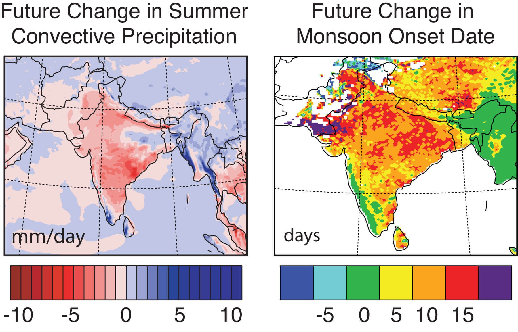
Returning to monsoon Asia — the setting of Lomborg’s exhortation for adaptation set in contrast to the efficacy of emissions reduction — uncertainty about the future course of the onset, strength, and intensity of the monsoon still reigns. While the AR4 models above suggest wetter summer monsoons (but dry winter monsoons), there is less certainty and more spatial variability. And regional climate models potentially give a different picture. Recently, researchers from Purdue University found that, in their climate model experiments, anthropogenic climate change ‘resulted in overall suppression of summer precipitation, a delay in monsoon onset, and an increase in the occurrence of monsoon break periods’

These maps show projected future changes in South Asian summer precipitation and monsoon onset date. A Purdue-led team found that rising future temperatures could lead to less rain and a delay in the start of monsoon season by up to 15 days by the end of the 21st century. (Diffenbaugh lab image) A publication-quality image is available at http://news.uns.purdue.edu/images/+2009/diffenbaugh-map.jpg
So, robust projections from climate models project future subtropical drying, including many areas with considerable vulnerability to climate change and water scarcity. For other regions, including monsoon Asia, uncertainty is still high.
I maintain that science matters for making sensible climate policy. If you get the science wrong, you might still accidentally stumble your way into good climate change policy, but adaptation and mitigation policies are more likely to be successful if they address accurately the most likely sources of vulnerability (fundamentals, like will a region get wetter or drier?). Therefore, undermining or mischaracterizing science in the name of one’s own ideological or policy goals seems likely to, in fact, undermine the chances of success of prescriptions for dealing with the consequences of anthropogenic climate change. Clean drinking water, sanitation, access to health care — all of these and more are good things irrespective of future climate change. The scientific details — in space and time and the sign and magnitude of uncertainty — matter, and no one is served well by getting them wrong.
UPDATE: I see Daniel Collins was thinking along similar lines.
Early anthropogenic influence on the climate system?
The Chronicle of Higher Education has a very nice review of Bill Ruddiman’s hypothesis that land use change by Holocene human populations had a detectable influence on climate and atmospheric chemistry prior to the Industrial Revolution. What I particularly like about this article is that it appears to successfully collect in a readable format the diverse array of evidence, opinions, and personalities involved in proposing, testing, and modifying this rather interesting hypothesis. Kudos to Josh Fischman for an enjoyable article.
Nested Comments
I’ve switched to using nested comments to try and maintain some flow for posts where there are a lot different ideas being knocked around. Alternatively I could try inline commenting. I’m going to see which method works best, so please bear with me as I try to optimize things
Yamal V: … but they pull me back in …
Via Jeff at his blog The Air Vent, in the midst of a post that includes a nontrivial quantity of ALL CAPS and multiple exclamation points (no <blink> tag?), the following statement (since that time stated in a more reasonable tone here):
For some reason EVERY RCS CORRECTION Briffa can conceive of refuses to turn upward to fit the ACTUAL data. This lack of flexibility in the RCS curves is what creates the HS.
I’m not sure why he doesn’t take my post on growth curves at Yamal seriously, but I’ve already explained why this is probably incorrect. The problem is an intermingling of the signal and the noise. As I showed previously, when I constructed an RCS curve using only the recent, living trees from Yamal, because these trees were growing roughly at the same time, and at that during a period of increasing temperatures, estimating a growth curve from them potentially intermingles the climate signal with the geometric growth curve.
One way to look at this is to consider only those trees that ceased growing prior to 1900. I’ve extracted these from the full Yamal set and estimated the regional curve standardization using a 67% spline. Here it is:

Let me be as clear as I can be, there is no sign that I can detect that it is old trees that increase their growth at Yamal (even if identified, this phenomenon would require some hypothesis as to the cause), At Yamal, a portion of the old trees are those that were growing together during a period of climate warming. If you examine the raw ring width, there are a few fossil series that have rapid increases toward the end. If Jeff’s hypothesis were correct, we’d expect these to be the oldest, right? In fact, the seven subfossil samples I identified as having rapidly increasing growth in their later years, six had a wide range of ages from 90 to 180 years (this comes with the caveat that we don’t know the exact pith age).
Furthermore, and as my earlier posts have shown, and as I’ll show again below, using a 67% spline (so that the later part of the regional growth curve bends slightly upward) you still get an increase in the chronology values during the 20th century.
Finally, what of the claim that combining the mean-detrended series demonstrates that the RCS method is invalid? One way we can test this is by first aligning all the ring widths by age (as was done here), observing where the curve of the juvenile grow trend flattens in the majority of trees (eyeballing it at around 175 to 200 years), throwing away the ring widths for the time when every tree was between 1 and 199 years of age (you get essentially the same result if you use 175 years), then realigning by time (year A.D.), and removing the mean. Lets look at the truncated growth curves in time and the mean of these series:

What immediately jumps out at you is that the mean for the most recent century and half is noticeably higher than the earlier part of the millennium. This doesn’t a priori indicate warmer temperature, but as I explained to Jeff here, once again there is the potential for this approach to remove climate signal in the process of detrending. For the most part, the mean following truncation is lower for the non-living trees at Yamal, but for the living 17 trees, the mean is similar or in some cases higher after truncation. Why? At least partially because after truncation the mean of the recent, living trees is of a large portion of the growth occurring during 20th century warming.
So, what do the chronologies look like if we use three different types of detrending? Let’s try constructing an RCS chronology using a 67% spline, negative exponential, and a generalized negative exponential curve:

The top shows the regional curve fit to all the raw Yamal data, the bottom panel zooms in on the part of the chronology since A.D. 1700 (heavy lines are 20 year low pass Butterworth filtered values). The regional curve fit that I think Jeff would endorse (67% spline) to fit his ‘U shape’ hypothesis actually results in slightly higher chronology values following the Little Ice Age, and slightly higher values at the end of the chronology in the mid 1990s.
My point is not to indicate a ‘correct’ method here — that goes well beyond ‘Blog Science’. Rather my point is this: detrending and standardization is one of the most challenging tasks in accurately estimating past low frequency climate variability from tree rings. Divergence is a serious challenge worthy of further study. What I don’t understand, however, is why methods or analyses (mean detrending, identifying growth curves from a small number of simultaneously growing trees) that can be shown to have the potential biases in specific instances that I’ve demonstrated here and in a previous post can still touted by those with a visceral dislike of paleoclimatologists as proof that another method is incorrect. If this debate was a collegial one that might be one thing, but there is nothing collegial — or scientific — about the language and tone from the other side. Too bad. To endorse once again Rob Wilson’s comment from Climate Audit:
“In fact, the fatal flaw in this blog and what keeps it from being a useful tool for the palaeoclimatic and other communities is its persistent and totally unnecessary negative tone and attitude, and the assumption that our intention is faulty and biased, which keeps real discourse from taking place.”
UPDATE: Minor grammar corrections
Briffa on Yamal
Keith Briffa and Tom Melvin have posted an interesting and thorough examination of the Yamal data here:
http://www.cru.uea.ac.uk/cru/people/briffa/yamal2009/
This now supersedes much if not all additional analysis I had considered for possible future posts.
Seeing Red (Noise): Galactic Cosmic Ray Fluxes and Tree Rings
First off, thanks to delayed.oscillator for inviting me to participate. I’m excited to be involved. Secondly, please forgive some of the formatting – I’m still new to this whole blogging thing. And away we go …
A recent paper (Dengel et al), published in the usually rigorous journal New Phytologist purports to show a statistically significant positive correlation between Galactic Cosmic Ray (GCR) fluxes and tree growth of sitka spruce (Picea sitka) from a plantation or managed forest in Scotland. Their hypothesis follows: High GCR fluxes stimulate aerosol nucleation in the atmosphere, leading to higher aerosol concentrations. The increased aerosol concentrations increase scattering of radiation, increasing the ratio of diffuse to direct radiation fluxes. The increased diffuse radiation penetrates more deeply into tree canopies, stimulating photosynthesis and growth.
Others have already shown that links between GCR fluxes and the Earth’s climate are quite dubious. Here we show that the conclusions drawn by the authors of this study are likely based on errors in their statistical analysis and faults in their study design.
The primary evidence in this paper for the GCR/diffuse radiation link to tree growth is tied to two Pearson correlations. One is a correlation between tree growth and March-August total diffuse radiation (n=45, r=+0.29, P=0.05). The second is a correlation between tree growth and GCR fluxes (n=45, r=+0.39, P=0.008). On the surface, both correlations appear to pass the traditionally accepted significance levels of P<=0.05, supporting the authors’ hypothesis.
The authors use a nominal sample size equal to 45, the total number of years in their dataset. This is fine, assuming that the underlying observations represent independent samples, e.g. a ‘white noise’ time series. To test this, we digitized the tree ring growth anomaly time series from the paper and estimated the lag-1 autocorrelation. If each observation were independent, the autocorrelation should be near 0. For this series, the autocorrelation is actually quite high (r=0.484) and significant (P=0.0008), indicating this time series has significant persistence (‘red’). The individual observations are not independent, and the significance of a Pearson correlation with n=45 will be overestimated.
This is easy enough to account for, however:

where n=original sample size, r is the autocorrelation of the underlying time series, and n’ is the new (effective) sample size. Plugging into this equation, we find that the sitka spruce tree growth time series has an effective sample size of only 16, instead of 45.
This change will not influence the actual correlation, but it will affect the test statistic used to determine statistical significance. For both correlations, we can recalculate the test statistic and significance level with the new effective sample size of 16:
GCR____ n T Statistic Significance
Original 45 2.7773 0.008
Revised 16 1.5647 0.139
Radiation n T Statistic Significance
Original 45 1.9870 0.050
Revised 16 1.1195 0.281
In both cases, the correlations now do not meet the criteria (P<0.05) to be considered statistically significant.
It is also very clear, from reading the paper, that the researchers were considering many, many possible associations — looking for a statistical correlation between the tree rings and some variable, regardless of whether there was a strong a priori theoretical basis to think there should be. Some of their correlations make sense – boreal summer temperatures concurrent with the growth year, for example, is reasonable since one would expect trees growing in Scotland could (possibly) be sensitive to temperatures during the growing season. Others are more tenuous, as when the authors attempt to correlate tree growth to diffuse radiation from the previous year.
In cases where one is data mining (as in this paper), it is important to guard against significant correlations that may be due simply to the overwhelming number of statistical tests made. Conceptually, it helps to think of the P value as your percent chance of a ‘false positive’, the chance that a statistically significant correlation is due to chance, rather than something meaningful. For most purposes, a P value of 0.05 (a 5% chance of a false positive) or less is considered acceptable. Each time you attempt another test, however, you increase the opportunity for this type of error. So, if two tests are conducted, the chance of a false positive, at a P=0.05 acceptable threshold, is actually 9.75% (assuming independent comparisons). In the case of total diffuse radiation, Dengel et al compared their tree growth time series against total diffuse radiation for each month of the current and previous growth years, a total of 24 tests (70.8% chance of a false positive). This makes it very likely that some of the correlations will be significant due to chance alone.
To adjust for this, researchers may use some flavor of what is called a Bonferroni correction, modifying the original P value to account for multiple comparisons. One simple way to do this is to divide your original acceptable threshold by the number of tests you conduct, increasing the burden of proof to accept a significant result. In the diffuse radiation example (tree growth versus diffuse radiation), that means a P=0.05 should actually be P=0.05/24=0.002. In other words, to have a P value confidence of 0.05, you actually need to meet a much stricter threshold, P=0.002. This burden is not met, either in the original analysis or with the adjusted sample size. The Bonferroni correction leads to less false positives (Type I errors), although it may increase the rate of false negatives (Type II errors).
Aside from not accounting for these features of their data and analysis, there are also some methodological oddities in the study design, where Dengel et al deviate from some standard practices in dendrochronology. First, they do not report many of the standard statistics used to assess the quality of a tree ring chronology-e.g. the mean interseries correlation (the common signal amongst trees) nor the mean sensitivity (a measure of a variable vs. complacent the ring width series). This makes it impossible for a reader to assess how well the trees correlate with each other, and whether the chronology really represents a common signal among the trees rather than simply an assemblage of noise. Second, they appear to use essentially randomly sampled trees from a managed forest. Normally, to find a tree (or set of trees) with a strong climate response researchers target trees where climate is the most limiting factor for growth. This often means trees near their climatic limits, where they may be stressed by temperature, moisture, or even radiation. Plantations or managed forests are typically not limited by these factors, because the goal is to manage growth for some purpose (e.g., timber, wildlife, et). Often this management can be quite intensive, involving fertilizer application, protection from pests, and thinning. Even at a location where tree growth is limited by climate, trees are not simply randomly sampled to try to find a climate signal. In particular, trees that may be influenced by competitive interactions with other trees (shading, etc) are generally avoided, because the signal in the tree rings will not necessarily best represent a response to larger scale climate variability. Randomly sampling trees through an even aged stand, as appears to be done in this study, will likely result in a large-scale signal that is equivocal or, worse, misleading. This is evidenced clearly by Figure 2 in the paper, where the authors attempted (largely unsuccessfully) to correlate tree growth against precipitation, temperature, and vapor pressure deficit. Dengel et al also use very short time series (only 45 years of growth), truncate the trees such that the juvenile growth is partially removed, and appear to use a relatively stiff spline in their detrending (potentially problematic in trees that may have experienced growth changes related to stand dynamics).
The criticisms I have made are not particularly nuanced or obscure, and are largely standard practice in climatology and dendrochronology. The lack of adherence to these practices likely led Dengel et al astray. I largely suspect their results will not be reproducible in other studies with a more typical design and analysis, but time will tell.

You must be logged in to post a comment.